Implementing Order-Independent Transparency
Hello! This will be a first attempt at coming back to writing some blog posts about interesting topics I end up rabbitholing about. All the older stuff has been sadly lost to time (and “time” here mostly means a bad squarespace website).
On-and-off I’ve been looking at some ways to handle transparency in my home code and just like the previous $N-1$ times I ended up wanting some sort of Order-Independent Transparency solution. However, time $N$ seemed as good of a time as any to actually try to implement something usable. So here are some ideas and the current state I’ve gotten to at the time of writing.
What is OIT? Why does it matter?
The reasoning for wanting Order-Independent Transparency comes from Order-Dependent Transparency being the way transparency rendering ends up being implemented in most computer graphics scenarios, and certainly in the majority of real-time rendering contexts.
The most natural way to achieve plausible-looking blending of transparent objects in computer graphics has been to draw the objects sorted from back-to-front. This is because when you’re drawing an object that’s partially letting you see what’s behind it, the easiest way to do it is to have the light (color) of the background already available so you can obscure it by some ratio, and then add the light of the object on top. This percentage is what people will often refer to as an “alpha”.
This imposes strict ordering when rendering all the objects in your scene to be farthest-to-closest, commonly referred to as the Painter’s Algorithm.
Well, it turns out we really don’t like that! This ordering spawns a myriad of problems that have annoyed us real-time rendering people for a while:
- This requires to sort everything that you’re going to draw based on distance to the camera. This has a performance cost in terms of doing the sort itself, but also in terms of doing the actual rendering. Without going into too much detail yet, current GPUs really really like to render the same kind of objects and the same kind of materials all at once. If you have to sort your objects, you can’t be rendering all your bottles first, then all your smoke particles, etc. If the order is bottle -> smoke -> bottle -> smoke, you need to draw them in that order.
- Even with correct sorting of all your objects, the results might still be incorrect! For example if an object is inside another object or if they overlap there would be pixels where an object should be rendered first and others where the other object should be rendered first. Think of an ice cube inside a glass of water.
- It can get really expensive to draw every pixel of all the transparent objects. Opaque rendering can easily optimize this by only really shading the closest opaque pixel that is visible in the end. With traditional back-to-front transparency this is not possible because the next object being rendered might need the result of the previous object since light is able to pass through it, therefore needing to render all of them. This situation where we draw into the same pixel more than once is referred to as overdraw. It’s easy to end up in situations where you have to shade and blend multiple screens worth of pixels, consequently killing performance.
An Order-Independent Transparency solution allows to render transparency in any order (shocker, I know). Most of the time OIT is thought about in the context of correctness, since scenes like the ice cube in the glass or smoke inside a car can look very jarring. In this sense, OIT would give fully a correct-looking end-result per-pixel.
However, depending on the implementation, it could also come with performance gains. The sorting of every object is now not required so that cost goes away, plus you’d be able to draw your transparent objects in whichever order is faster (e.g. all of the same objects/materials drawn together). Some solutions even allow to cut on overdraw, since they can avoid drawing transparency that would never be visible because there’s other transparent objects in front that fully occlude it.
Finally, I personally consider the possible simplicity gains on the whole codebase to be important. Without OIT, you often end up with complicated interfaces that have to take transparent draws from a bunch of systems, sort them and then dynamically dispatch the draws in the correct order, with callbacks to each system’s custom code, etc. With some OIT solutions you might be able to write conceptually simpler and more performant code such as:
draw_ghosts();
draw_particles();
draw_glasses_of_wine();
draw_the_ice_cubes_in_the_glasses_of_wine();
draw_whatever_other_transparent_draws_with_a_very_fancy_shader();
Polychrome Transmittance
When we say that light is “going through a surface” there’s two broad ways in which we can categorize this.
If the matter of the medium is mostly opaque but it’s leaving room for the light to pass through unencumbered we would call this phenomenon partial coverage. You can think of this sort of surface as having “tiny holes” where the some of the light can sneak through without ever interacting with it. Examples of this could be some fabrics or meshes of some kind.
When light is going through a medium then we would call that transmission. Here light interacts with the medium in more complex ways than just passing through or not. Notably, for our purposes, the medium could be letting some frequencies of light through more than others. Examples of this could be liquids, plastics, etc.
Both of these are really well explained by Morgan McGuire in his this part of his presentation about transparency in Siggraph 2016
Partial coverage is what we’ve mostly been modeling in real-time rendering and what most people is talking about when mentioning alpha blending or alpha compositing. In this case we simply occlude light by a single “alpha”, the ratio of light that’s blocked.
But if we only model partial coverage this doesn’t accurately represent all those other types of media such as transparent colored plastics, tinted glass, some liquids, etc. And this is a real shame since we’re missing out on all the eye-candy that transmission would have given us.
This is why for my transparency solution I wanted to support polychrome transmittance, where we’d handle how light is getting transmitted differently in multiple frequencies. Aaaaand of course these frequencies will be just red, green and blue because this is real time graphics and those are the ones we mostly care about anyways.
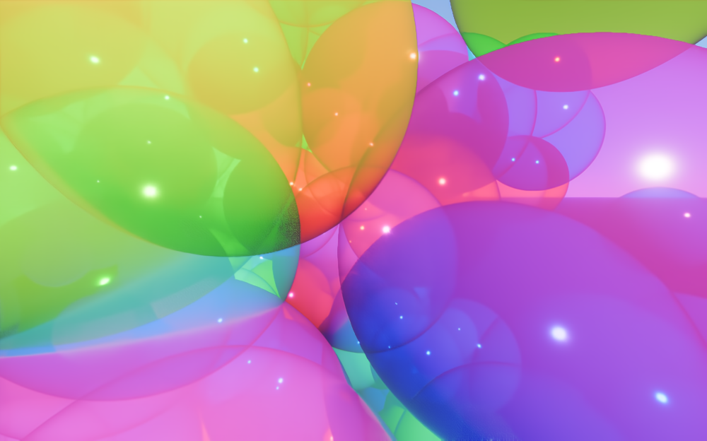
For the purposes of an implementation, polychrome transmittance could be considered a superset of partial coverage, since we could always just say that light is being transmitted by the same ratio in all light components, hence simulating the behavior partial coverage. Here is how our test scene would look like if simulating partial coverage via monochrome transmittance:
However, handling polychrome transmittance can impose extra requirements compared to traditional monochrome alpha, which would only require us to handle how the visibility of a single channel changes. In a way, it can even triple the computation and even potential memory requirements of an OIT solution. A lot of OIT solutions could be made cheaper or at least be simplified if only monochrome transmittance is desired by simply running the logic and storing single values instead of three.
How I didn’t do it
There’s a few ways to approach OIT that I didn’t quite like the trade-offs of. This doesn’t mean they aren’t the right approach for your use-case, or even that they won’t become the one true way to go in the future as the landscape of real-time rendering evolves.
Raytraced Transparency
Here you simply trace a ray against all your transparent geometry while accumulating transmittance and luminance (or radiance if you wanna get radiometric). When you shade something, you multiply the resulting luminance by the current transmittance and accumulate the transmittance to use on the next point to shade. After there’s nothing left to hit, you read the luminance of your opaque layer and obscure it with the accumulated transmittance. Something like this:
float3 luminance = 0.0;
float3 transmittance = 1.0;

Ray ray = init_ray_from_eye_into_the_scene(/*...*/);
while (ray.hit_stuff())
{
    Shaded_Hit hit = shade(ray);
    luminance += hit.luminance * transmittance;
    transmittance *= hit.transmittance;
}

float3 opaque_layer_luminance = backbuffer.Sample(/*...*/);
return luminance + (opaque_layer_luminance * transmittance);
This is nice to read, and even if it looks very didactic, a real implementation can look pretty much like that. It also supports extra phenomena like refraction very naturally. In principle I really like this.
The main issue is with how much heavy lifting that shade(ray) call is doing. This needs to handle shading of any type of transparent surface you want to have in your renderer, the same code-path would need to be able to shade materials that range from opaque glass geometry to smoke particles.
This requires that you make a single shader that supports all the different shading models you need, and it’ll get fatter and slower as time goes on (hurting code size, register usage, etc.). And you are still effectively shading things in the order they are per-pixel, meaning that you can’t do any optimizations where you batch per-shader/material.
There’s other limitations, like keeping an acceleration structure for all your transparent geometry (including particles), but depending on the context these are manageable.
That said, if you can keep the complexity of this shading path in check, this might be a solution to consider. Even more if hardware and graphics APIs evolve towards handling this type of branching better.
Per-Pixel Lists
The idea here is also simple, you render all your transparency however you want, but instead of blending it to the screen, you add it to some sort of list that you keep for each pixel. You’d need to add the luminance, the transmittance and the depth:
float3 luminance     = /*...*/
float3 transmittance = /*...*/
float  depth         = /*...*/
add_to_list(luminance, transmittance, depth);
After you’re done, you take this list, sort it based on the depth and add up all the results in a loop that looks kind of similar to the raytracing one:
sort(list); // Could be in place, in a separate pass, or even done as you're adding elements to the list

float3 luminance     = 0.0;
float3 transmittance = 1.0;
for (int i = 0; i < list.count; ++i)
{
    luminance += list[i].luminance * transmittance;
    transmittance *= list[i].transmittance;
}

float3 opaque_layer_luminance = backbuffer.Sample(/*...*/);
return luminance + (opaque_layer_luminance * transmittance);
This works well, and it lets you render all transparency in any order you want, batching to your heart’s content. The main problem here is that these lists can get very big and you need to account for a single pixel having many transparent surfaces wanting to contribute to it. It’s not unlikely at all to have a stack of 20+ particles on top of each other, all faint enough that you can still see through all of them. The longer these lists can get, the more time time will be spent sorting them and the more memory they would require.
Let’s say you’re rendering at 1440p, maybe you encode luminance in R9G9B9E5, transmittance in R8G8B8 plus depth in a single float16. That’s 9 bytes per item on the list. If you want to support 16 elements per-pixel that’s $\frac{2560\times1440\times9\times16)}{(1024\times1024)} = 506.25$ MB which is half a GB for just the lists. Plus you’d need to make these ~3.6 million lists sorted, either as you add or with a separate sorting pass afterwards. And 16 elements might look like many, but it’s not hard to reach at all if doing particles.
There’s many flavors of this, keeping linked-lists, only considering the closest N elements, having all items come from a shared buffer for all pixels, etc. Due to the nature of having to keep a list, they all inherently require the memory necessary to hold and sort as many items as you’ll need.
If the need to handle many overlapping transparent surfaces is not a requirement for you though, this might be worth considering!
How I did do it
The key problem of achieving order-independence is that when you render a surface you don’t know what could be in-between that surface and your eye. You just don’t have the information about how much light from the surface you just shaded is going to make it to the viewer.
This is made explicit in the code for raytraced transparency, every time you shade a surface you have the variable transmittance holding quite literally the ratio of how much light any surface we find at that moment is going to reach the eye.
It would be really good if we could just™ know the transmittance of the path in front of the surface we’re shading. The approach I’ll describe here attempts to do essentially that. It generates a function of transmittance over depth per-pixel. This then can be used to render transparency while occluding the luminance that reaches the eye by sampling that function.
This is what approaches like Moment Transparency or Moment-Based Order-Independent Transparency do. The challenge here is to create this function of transmittance over depth in a way that’s accurate and still doesn’t break the bank in terms of performance, memory usage, etc.
The simplest form of this idea would involve two passes, first generating the transmittance-over-depth function that we’ve mentioned, then do a second pass where we render all the transparency using the transmittance information at each point. That said, to help with the representation of transmittance it’s useful to render depth bounds so we can distribute its precision to where there’s going to be relevant information.
The representation I’m using to generate this transmittance-over-depth function, and the general approach, is the one from Wavelet Transparency where they use Haar wavelets to encode it. I can’t recommend this paper enough and if you want to dive deep into the mathematics of how you can use wavelets to represent monotonically non-increasing functions like this, definitely go give it a read! This representation I’m sure can be useful for many other applications.
Wave-what?
To give a back-of-the-napkin explanation of wavelets it’s easier if we start with Fourier series. With them you can represent a function as a sum of sinusoidal waves, so you can encode your annoyingly infinite function as a set of coefficients that represent these individual waves. This transformation process is called the Fourier Transform. With only a few coefficients you can get a pretty good representation of the original function which you can store, process, sample later, etc.
So why not use this to represent our transmittance? Well these are kind of bad at representing localized events in a function. And transmittance over depth changes sharply at arbitrary points.
Fourier series being bad for this makes some intuitive sense since you’re adding these infinite waves on top of waves at every $t=(-\infty, +\infty)$. If you then wanted to represent a sharp unique change in the middle of the function and nowhere else it’s not easy to see what waves you could add to do so. If this sounds foreign, there’s an amazing explanation of Fourier series by 3Blue1Brown here.
Here you can see what happens if we just add the top three sinusoidal functions together, we get this nicely continuous function, but it would be really hard to represent a particular shape in the middle of it.
Wavelet bases also represent signals through the amplitude of some coefficients, but this signals are localized in time, they are quite literally a “little wave” at specific $t$. By composing these piece-wise signals we can represent localized phenomena much easier and with much less coefficients. You can see here how if we add these three top wavelets together we can represent something way more localized in time.
This example is using Morlet wavelets but there’s many more you could use. One of them being the Haar wavelets that the paper uses. The coolest among them being the Mexican hat wavelet of course.
Another hugely recommended watch that introduces signal processing, time and frequency domains, Fourier and then wavelets is Artem Kirsanov’s video on Wavelets. The book A Wavelet Tour of Signal Processing was also really good. The first chapter is available for free and does a good job of introducing some of these concepts.
Hopefully this gives some intuition of what’s happening when we try to encode the arbitrary function of transmittance over depth (depth being our “time” axis) using wavelets. This is a huge field and one that requires to build on previous knowledge at many steps. If you want to understand this better I recommend giving the references linked above a read/watch and then go back to the paper to see how it’s used in practice.
With this in hand, we can go into how the different passes will generate and use this wavelet representation.
Computing Depth Bounds
I start with rendering transparency draws outputting linear depth, keeping the minimum and maximum values for each pixel. There’s nothing particularly interesting about this pass, I’m rendering to a two component target with a blend-state that just keeps the maximum value, then just something simple like the following will do:
float2 pixel_shader(float4 clip_position)
{
    float linear_depth = device_depth_to_linear_depth(clip_position.z);
    return float2(-linear_depth, linear_depth); // Storing negated minimum distance so "max" blending keeps the right values
}
You could store device depth instead and avoid the extra transformation, but have in mind that depending on how you’re handling your device depth, normalizing a depth value to use with your transparency might need to account for it being non-linear.
For our example scene in this post, the depth bounds look like this, with minimum and maximum respectively. The visualized range here goes from 35 to 140 meters so it’s clearer to see a black-to-white value.
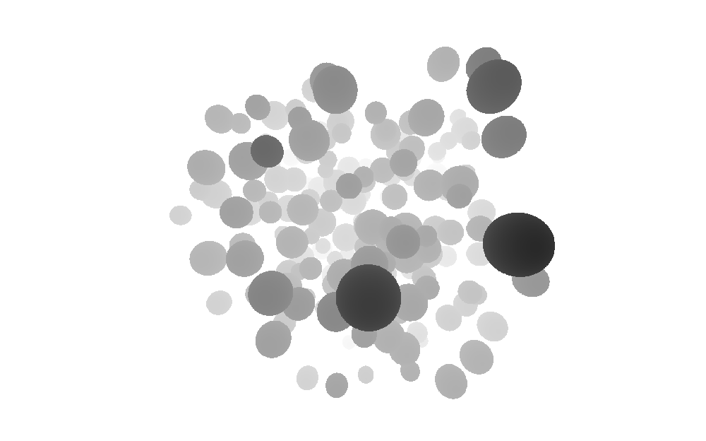 |
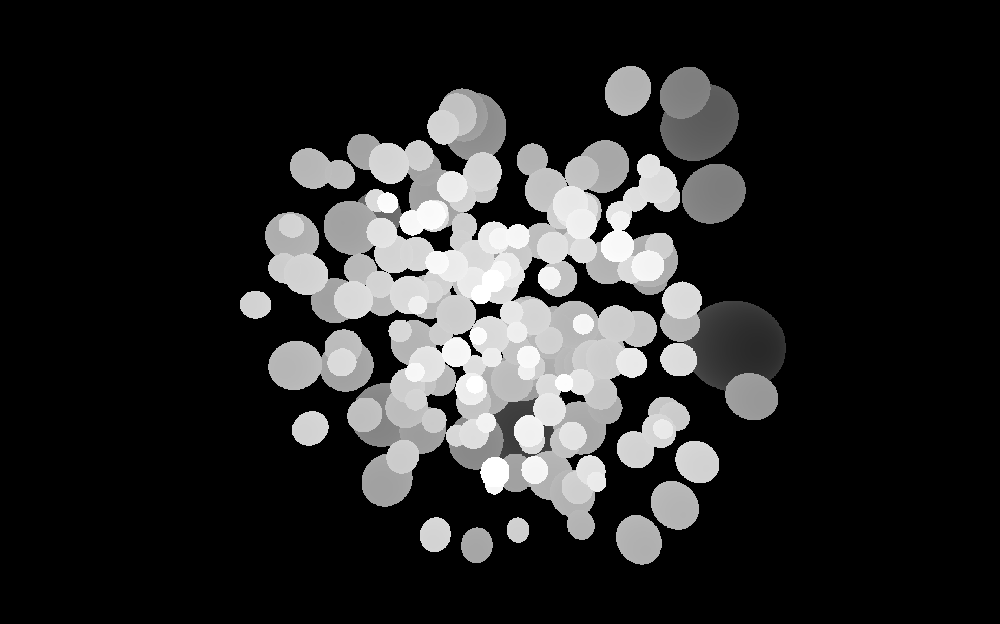 |
This extra pass might be a concern if you’re going to be rendering a lot of transparency, or if your draws involve expensive computations for just outputting depth (e.g. heavy vertex shader animation). However, since all we want to do here is to bound the space per-pixel where we’re writing alpha, you could easily do lower detail draws or even simple bounding boxes or spheres. You could even render the bounds at a lower resolution to help with bandwidth and memory costs.
Generating Transmittance
In this pass, I’m rendering all the transparency through a shader that only outputs transmittance, which is cheaper than fully shading them. From the given transmittance and depth, a given set of coefficients are generated, which are added to the existing coefficients stored in a render target. The shader would be running something like this:
void pixel_shader(float4 clip_position)
{
    float depth         = /*...*/;
    float transmittance = /*...*/;
    add_transmittance(clip_position.xy, depth, transmittance);
}
At the time of writing I’m storing the coefficients in a texture-array at render resolution. The number of coefficients (length of the texture array) is determined by the rank of the Haar wavelets where rank $N$ requires $2^{N+1}$. For this blog post I was using rank 3, but lower ranks are a very sensible approach for a big reduction in texture size (and hence less memory usage, bandwidth, etc.).
An important note in this regard is that a single transmittance event doesn’t need to write to all the coefficients, only to $Rank+2$ of them, so even at higher ranks it’s not as bandwidth intensive at it would initially seem. Similarly, when sampling later only $Rank+1$ coefficients are necessary for a single sample.
These coefficients are positive floating point numbers possibly outside the 0-1 range, so an appropriate format is required. I’m using R9G9B9E5 which shares a 5-bit exponent between the three 9-bit mantissas for red, green and blue, each of the channels for RGB transmittance. If you only wanted to do monochrome transmittance you could simplify this to a smaller format that only stores a single floating point value, or swizzle them together and reduce the texture-array length.
The key feature that makes this part order-independent is that the coefficients are purely additive. It might be obvious to some readers, but what is breaking order-independent in classic methods is that the order of operations affects the result, so if you’re doing traditional alpha blending (denoted here by $\diamond$), it’s not the same doing $(a \diamond b \diamond c)$ than $(b \diamond a \diamond c)$. However, since we’re only adding coefficients together, we would get the same result doing $(a + b + c)$ and $(b + a + c)$ due to addition being commutative (besides possible floating-point representation differences).
Here is a visualization of the transmittance (sampled at far-depth) when adding each of the spheres in the example scene. You can see how the order in which they are being added is arbitrary.
Something you would encounter while implementing this with the same setup, is that R9G9B9E5 cannot be used as a render target to output to (in D3D12 at least). So we need to perform the addition manually. Sadly we can’t simply InterlockedAdd into them either. To solve this, what I’m doing is casting the R9G9B9E5 to a R32_UINT target and doing a Compare-And-Swap loop to read the value, increment it by the addend and store it again atomically. This could look something like this:
int    coefficient_index  = /*...*/;
float3 coefficient_addend = /*...*/;

RWTexture2DArray<uint> texture = /*...*/;
int2 coordinates = /*...*/;
int3 array_coordinates = int3(coordinates, coefficient_index);
int attempt = 0;
uint read_value = texture[array_coordinates];
uint current_value;
do
{
    current_value = read_value;
    uint new_value = pack_r9g9b9e5(unpack_r9g9b9e5(current_value) + coefficient_addend);
    if (new_value == current_value) break;
    InterlockedCompareExchange(texture[array_coordinates], current_value, new_value, read_value);
}
while (++attempt < 1024 && read_value != current_value); // Without the attempt check, DXC was generating horrific code, many orders of magnitude slower than with it for some reason
For the transformation of transmittance and depth into the additive coefficients, and the code to later sample the resulting coefficients into a transmittance at a given depth, you should go read the original Wavelet Transparency paper. There’s more details about the process described here and a better explanation than what I could ever do here.
However, I’ll put here my simplified version of the code to generate and sample coefficients I used for this post. Huge thanks to Max for his blessing and please go read their paper!
I’ll leave out of the snippets the coefficient addition and sampling, the addition would be something like the logic above, or any replacement that allows safe accumulation into the different coefficients. The sample would most likely be just a traditional texture sample. With that said, my coefficient generation code goes as follows:
template<typename floatN, typename Coefficients_Type>
void add_event_to_wavelets(inout Coefficients_Type coefficients, floatN signal, float depth)
{
    depth *= float(TRANSPARENCY_WAVELET_COEFFICIENT_COUNT-1) / TRANSPARENCY_WAVELET_COEFFICIENT_COUNT;

    int index = clamp(int(floor(depth * TRANSPARENCY_WAVELET_COEFFICIENT_COUNT)), 0, TRANSPARENCY_WAVELET_COEFFICIENT_COUNT - 1);
    index += TRANSPARENCY_WAVELET_COEFFICIENT_COUNT - 1;

    [unroll]
    for (int i = 0; i < (TRANSPARENCY_WAVELET_RANK+1); ++i)
    {
        int power = TRANSPARENCY_WAVELET_RANK - i;
        int new_index = (index - 1) >> 1;
        float k = float((new_index + 1) & ((1u << power) - 1));

        int wavelet_sign = ((index & 1) << 1) - 1;
        float wavelet_phase = ((index + 1) & 1) * exp2(-power);
        floatN addend = mad(mad(-exp2(-power), k, depth), wavelet_sign, wavelet_phase) * exp2(power * 0.5) * signal;
        coefficients.add(new_index, addend);

        index = new_index;
    }

    floatN addend = mad(signal, -depth, signal);
    coefficients.add(TRANSPARENCY_WAVELET_COEFFICIENT_COUNT - 1, addend);
}
The counterpart of that code would then take the array of coefficients and evaluate them at a given normalized depth, which you can see in the following snippet:
template<typename floatN, typename Coefficients_Type>
floatN evaluate_wavelet_index(in Coefficients_Type coefficients, int index)
{
    floatN result = 0;

    index += TRANSPARENCY_WAVELET_COEFFICIENT_COUNT - 1;
    [unroll]
    for (int i = 0; i < (TRANSPARENCY_WAVELET_RANK+1); ++i)
    {
        int power = TRANSPARENCY_WAVELET_RANK - i;
        int new_index = (index - 1) >> 1;
        floatN coeff = coefficients.sample(new_index);
        int wavelet_sign = ((index & 1) << 1) - 1;
        result -= exp2(float(power) * 0.5) * coeff * wavelet_sign;
        index = new_index;
    }
    return result;
}
template<typename floatN, typename Coefficients_Type>
floatN evaluate_wavelets(in Coefficients_Type coefficients, float depth)
{
    floatN scale_coefficient = coefficients.sample(TRANSPARENCY_WAVELET_COEFFICIENT_COUNT - 1);
    if (all(scale_coefficient == 0))
    {
        return 0;
    }

    depth *= float(TRANSPARENCY_WAVELET_COEFFICIENT_COUNT-1) / TRANSPARENCY_WAVELET_COEFFICIENT_COUNT;

    float coefficient_depth = depth * TRANSPARENCY_WAVELET_COEFFICIENT_COUNT;
    int index = clamp(int(floor(coefficient_depth)), 0, TRANSPARENCY_WAVELET_COEFFICIENT_COUNT - 1);

    floatN a = 0;
    floatN b = scale_coefficient + evaluate_wavelet_index<floatN, Coefficients_Type>(coefficients, index);
    if (index > 0) { a = scale_coefficient + evaluate_wavelet_index<floatN, Coefficients_Type>(coefficients, index - 1); }

    float t = coefficient_depth >= TRANSPARENCY_WAVELET_COEFFICIENT_COUNT ? 1.0 : frac(coefficient_depth);
    floatN signal = lerp(a, b, t); // You can experiment here with different types of interpolation as well
    return signal;
}
Note that you can get some good gains by further optimizing this, especially by combining the multiple calls to evaluate_wavelet_index(...) into the same loop, thus avoiding redundant samples. But the versions further optimized are a bit less clear and they can be a great candidate for a further post about squeezing this further and making it faster 🦹. That said, an example further along in this post shows evaluate_wavelets with the merged loops 😉.
The code above could encode any additive signal, so they could be used for other purposes as well. Something worth pointing out too is that depth here is already normalized between the transparency min and max depth bounds. With that in mind, here’s a couple wrappers to add and sample transmittance specifically:
template<typename floatN, typename Coefficients_Type>
void add_transmittance_event_to_wavelets(inout Coefficients_Type coefficients, floatN transmittance, float depth)
{
    floatN absorbance = -log(max(transmittance, 0.00001)); // transforming the signal from multiplicative transmittance to additive absorbance
    add_event_to_wavelets(coefficients, absorbance, depth);
}

template<typename floatN, typename Coefficients_Type>
floatN evaluate_transmittance_wavelets(in Coefficients_Type coefficients, float depth)
{
    floatN absorbance = evaluate_wavelets<floatN>(coefficients, depth);
    return saturate(exp(-absorbance)); // undoing the transformation from absorbance back to transmittance
}
Transmittance Function Examples
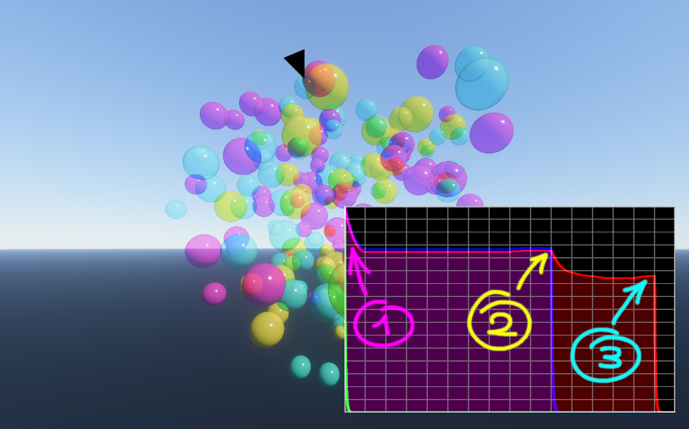
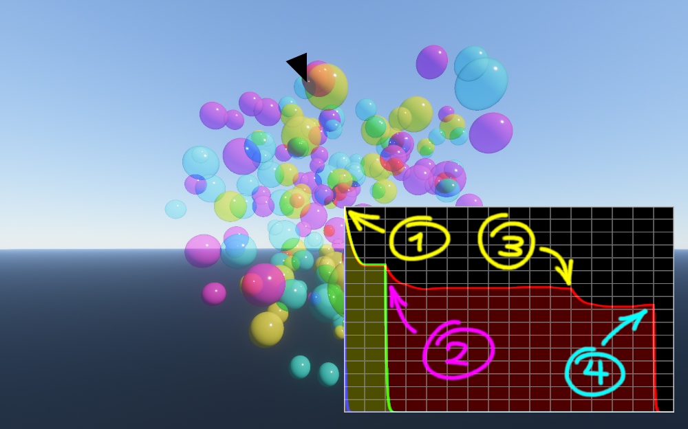
After adding up all the coefficients, we effectively have recreated the full function of transmittance over the depth. Let’s look at some pixels that range from having 1 to 4 surfaces to see how the transmittance falls at the depths where the surface is. Note that this is plotting the transmittance over the normalized depth within the depth bounds we have computed in the beginning, which means that towards the left, transmittance will always be $(1,1,1)$ and towards the right it will always be the same as the last value plotted.
In the left image there is a single magenta ball, which has a transmittance of $(1,0,1)$ because it’s letting through the red and blue channels, while fully occluding green light. The plot is showing how the green light quickly goes to zero and all that’s left is a slightly darkened magenta.
To the right of it you can see two overlapping cyan balls, with a transmittance of $(0,1,1)$. These show how multiple overlapping surfaces of the same color keep decreasing transmittance at each event, so the transmittance after both of them is an even darker cyan. This is what we would expect, the first ball is occluding all red light, and letting through a percentage of the green and blue. Then the second ball is occluding the remaining green and blue light by yet another percentage (and fully occluding red light, but that was already zero).
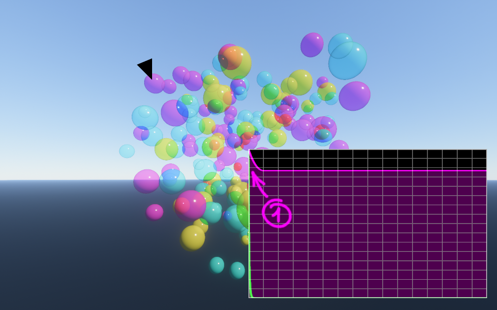 |
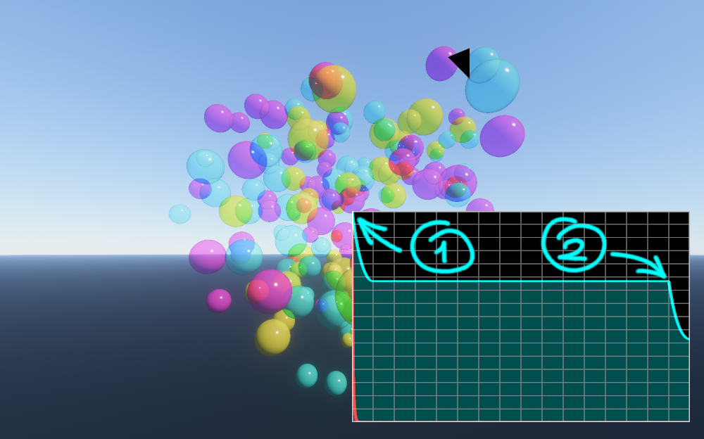 |
Here there’s a couple of more complicated cases. First one where there is a magenta, yellow and cyan ball in that order. In this case, each are letting through only 2 of the red, green and blue channels. After light has gone through all 3, every channel must have been fully occluded at some point, so no light can possibly be going through all 3 balls, hence the transmittance falling to zero at the end of the plot.
This also hints at why I chose these colors for the balls in the example scene, it makes it easier to visualize how the 3 channels fall if we use the 3 primary colors of a subtractive color system, since they naturally generate known results when combined, and eventually zero/black.
 |
 |
Shading Transparency
Now we can go over the transparency draws in a “traditional” forward-rendering way, shade them fully and occlude them by the transmittance in front before blending them in.
We’re rendering our transparent draws on top of the fully shaded opaque layer, so we would first need to obscure the opaque layer by the transmittance of every transparent draw in front, this could be done with a full-screen pass in various ways. An easy one would be to set up multiplicative blending and do the following:
float3 fullscreen_pixel_shader()
{
    float4 clip_position = /*...*/;
    float depth = +FLOAT32_INFINITE;

    float3 transmittance_in_front_of_opaque_layer = sample_transmittance(clip_position.xy, depth);
    return transmittance_in_front_of_opaque_layer; // final_rgb = this.rgb * render_target.rgb
}
After running a shader like the above, the opaque layer with the applied transmittance on top of it would look as follows on our example scene:
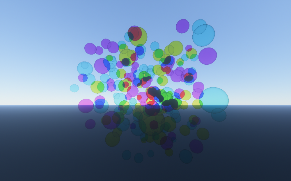
Then I go over then transparent draws in any order. Now the blending can be fully additive since we’re only adding the light that the current draw is contributing to the final image. The necessary occlusion for the current draw is handled by the transmittance_in_front, and the occlusion of whatever is behind the current draw will be handled by those draws that are behind whenever they do their shading.
The code for these draws could look like the following, with a purely additive blending state:
float3 pixel_shader(float4 clip_position)
{
    float  depth           = /*...*/;
    float3 lighting_result = /*...*/;

    float3 transmittance_in_front = sample_transmittance(clip_position.xy, depth);
    return lighting_result * transmittance_in_front; // final_rgb = this.rgb + render_target.rgb
}
Similarly to the transmittance, we can visualize how the spheres now get rendered in an arbitrary order. Each of them adding their light occluded by whatever is in front. Note how this visually resolves ordering due to how we’re interpreting whatever is more occluded as being behind and vice-versa.
And after this, we’re done! Every draw is contributing to the final image by the right amount, and all the passes we’ve done could have rendered each transparency draw in any order.
Extra Sauce
Overdraw Prevention
We’ve also gone through not-that-much all this pain to generate our transmittance-over-depth function, why not take advantage of it? Here is a good way I found to put it to good use.
After we’ve generated the transmittance, we can take a look at the resulting function and see if it ever becomes zero, if it does, that means that nothing after that point in the depth range is visible, so let’s just write to a depth buffer and use that for doing transparency shading!
Opaque rendering does just this, because you know that the transmittance after a fully opaque pixel is zero, you can happily write depth and after that, you don’t need to do any shading for depths that lay behind. Transparency rendering is a super-set of that, where transmittance is not binary, but once it’s zero, we’re at the same situation.
By writing depth and testing against that depth we’re avoiding potentially a lot of shading that would have been useless. This is a classic problem with transparency, you have 30 smoke particles that are so dense that you only see the closest 5 or 6 layers, but if you’re following a traditional transparency pipeline you’re having to shade them all. All that work shading the first few ones was wasted, since none of that contributed to the final image.
To do this, after the transmittance generation step, you could run a full-screen draw like the following, where we look for a depth at which it’s safe to consider transmittance to be so low that anything behind won’t contribute to the final result. This could of course be done in many other ways, but the general idea remains the same:
float pixel_shader() : SV_DEPTH
{
    float4 clip_position = /*...*/;
    float threshold = 0.0001;

    //
    // If transmittance an infinite depth is above the threshold, it doesn't ever become
    // zero, so we can bail out.
    //
    float3 transmittance_at_far_depth = sample_transmittance(clip_position.xy, +FLOAT32_INFINITY);
    if (all(transmittance_at_far_depth <= threshold))
    {
        float normalized_depth_at_zero_transmittance = 1.0;
        float sample_depth = 0.5;
        float delta = 0.25;

        //
        // Quick & Dirty way to binary search through the transmittance function
        // looking for a value that's below the threshold.
        //
        int steps = 6;
        for (int i = 0; i < steps; ++i)
        {
            float3 transmittance = sample_transmittance(clip_position.xy, sample_depth);
            if (all(transmittance <= threshold))
            {
                normalized_depth_at_zero_transmittance = sample_depth;
                sample_depth -= delta;
            }
            else
            {
                sample_depth += delta;
            }
            delta *= 0.5;
        }

        //
        // Searching inside the transparency depth bounds, so have to transform that to
        // a world-space linear-depth and that into a device depth we can output into
        // the currently bound depth buffer.
        //
        float device_depth = device_depth_from_normalized_transparency_depth(normalized_depth_at_zero_transmittance);

        return device_depth;
    }

    return 0;
}
Note how here we have to do if (all(transmittance <= threshold)) meaning that we’re checking that all the components of our polychrome transmittance have become zero. If all components are not zero it means that there’s still some light frequencies that can be visible behind a given depth.
Here is a visualization of where this code has written depth due to finding a point at which transmittance became zero. You can see how this triggers in the areas where multiple spheres overlap, especially if they are different colors because they would each be occluding light from different frequencies.
In the checkerboard pixels, we are avoiding doing any shading for some of the transparent surfaces that lay after a certain depth.
Occluding Opaque Layer
We can extend this previous idea further. If we generate transmittance before we do the shading of our opaque layer, it means that we know about this transmittance-over-depth when we’re shading the opaque layer as well. So first thing we can do is to also sample this transparency depth we wrote and avoid shading the opaque draws that will be fully occluded by transparent draws.
This requires the slightly unusual approach of doing a lot of your transparency rendering before your opaque stuff, but there’s not much going against that. One thing that’s useful to do before any transparency rendering is to get some sort of depth you can use. Lots of renderers already do a depth-prepass, or a GBuffer or generate a VBuffer (visibility buffer), etc. All of which generate a depth buffer before doing any shading.
In my case I render a visibility buffer first (including depth), then I generate the transmittance and write depth at zero transmittance (to a separate depth buffer, cause you probably want to keep the opaque-only depth buffer for other stuff). The I use that to test against when shading both the opaque layer and the transparent draws.
This adds some more savings to those pathological cases for transparency mentioned in the previous section. However, if transmittance is not quite reaching zero you can still put this information to good use, for example, by using variable-rate shading to make those pixels cheaper, since they’re going to be partially occluded anyway and might not need that high-frequency detail.
Separate Compositing Pass
Instead of rendering directly on top of the shaded opaque layer, you can render to a separate target instead and composite transparency on top of opaque in a separate pass.
This decouples transparency rendering from opaque almost completely. We’re still using the opaque layer’s depth buffer to initially test against but this is often already available even before opaque shading in any sort of “deferred” renderer. Forward renderers still often have a depth pre-pass that we could use as well.
This opens the possibility of rendering transparency at a lower resolution than opaque, this could even be made dynamic depending on the cost of transparency in a given scene. This could help handle classic frame-time spikes that happen when lots of low-frequency detail transparency fills the screen, such as big explosion or smoke effects.
Also allows to run dedicated full-screen passes on the transparency results only. For example extra transparency anti-aliasing or de-noising.
During compositing, I’m also seeing how much the opaque result is different from the composited final result and storing that in the alpha channel of the result lighting buffer. This can be used as a value that represents how much of the opaque layer is visible, which comes in handy tremendously during Post-FX, especially for things that rely on motion vectors and/or depth from the opaque draws such as temporal anti-aliasing, depth-of-field, etc.
This is also good to pass to various up-scaling technologies in the market to allow them to handle transparency more appropriately. A good example of this are the reactive and transparency masks for AMD’s FidelityFX Super-Resolution.
Deferring the blending on top of the opaque layer also opens up the possibility of writing extra data during the shading pass to do more effects during composition. For example we could output a diffusion factor or refraction deltas like Phenomenological Transparency does and apply those effects at the compositing stage.
Something that should be noted is if you’re doing memory aliasing of the rendering resources used throughout your frame, you might want to move things around. What you wouldn’t want is to have the big coefficients array be kept alive during all your opaque shading passes. If you do want to generate transmittance before opaque shading, it’s a good idea to resolve transparency before opaque as well and store all you need to do during the final compositing pass after you’ve shaded the opaque layer. This would make the largest memory requirement to be quite short lived in the frame, likely reducing the upper bound for memory requirements.
A way to separate the passes would be to just remove the pass that previously occluded the opaque layer. Then have the transparency draws output something on their alpha channel to see where they wrote something.
float4 pixel_shader(float4 clip_position)
{
    float  depth           = /*...*/;
    float3 lighting_result = /*...*/;

    float3 transmittance_in_front = sample_transmittance(clip_position.xy, depth);
    lighting_result *= transmittance_in_front;

    return float4(lighting_result, 1.0);
}
And we can use this result, along with this alpha channel to help us early out in the compositing pass, which looks something like this:
float4 fullscreen_pixel_shader()
{
    float4 clip_position = /*...*/;

    float4 transparent_layer = sample_transparency_result(clip_position.xy); // Potentially lower resolution
    if (transparent_layer.w > 0.0)
    {
        float3 transmittance_in_front_of_opaque_layer = sample_transmittance(clip_position.xy, depth);

        float3 opaque_layer = sample_opaque_result(clip_position.xy);
        float3 composited_light = (opaque_layer * transmittance_in_front_of_opaque_layer) + transparent_layer.rgb;

        float approximate_opaque_layer_visibility = luminance(transmittance_in_front_of_opaque_layer); // Could be done in a million other ways, depending on the usage

        return float4(composited_light, approximate_opaque_layer_visibility);
    }
}
Applying noise to transmittance
As much as the wavelet coefficients do a great job of representing transmittance, they can suffer from imprecision especially when a transmittance event falls in between certain depth ranges, even more so the lower the wavelet’s rank. To get around this I’m injecting the left half of triangle noise both when writing transmittance and when sampling it.
It only injects noise that moves the depth location towards zero, to avoid transmittance events self-occluding. This noise is also not applied towards the extremes of the depth function. Done via sampling a tent-like function with the normalized depth.
More investigation could be done about where is the best place to inject noise, and which type of noise is the best for this purpose (e.g. blue noise tends to be just™ good at all these things).
Depending on the type of noise, strength, frame-rate and even type of scenes, it might be beneficial to run a dedicated de-noising pass on the transparency results. This would be made possible by decoupling transparency results from opaque and compositing later, as explained in the previous section. Alternatively, it might be that an existing Temporal Anti-Aliasing pass in your renderer would already be doing a good job of softening that noise.
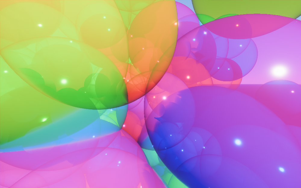
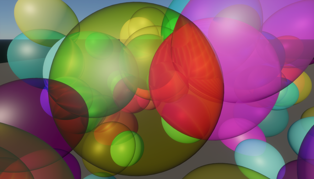
This is an example of a scene that has a ton of overlap in a way that forces these artifacts, and how it looks when injecting noise on the transmittance function input followed by the denoised result. You might want to open these in a new tab to get a better look!
| Raw | With added noise | Denoised |
 |
 |
 |
Avoiding Self-Occlusion
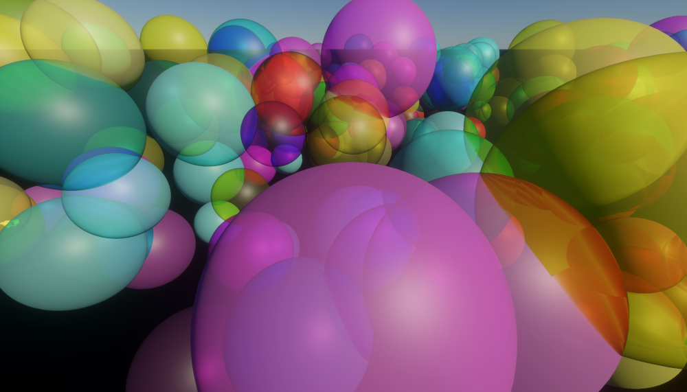
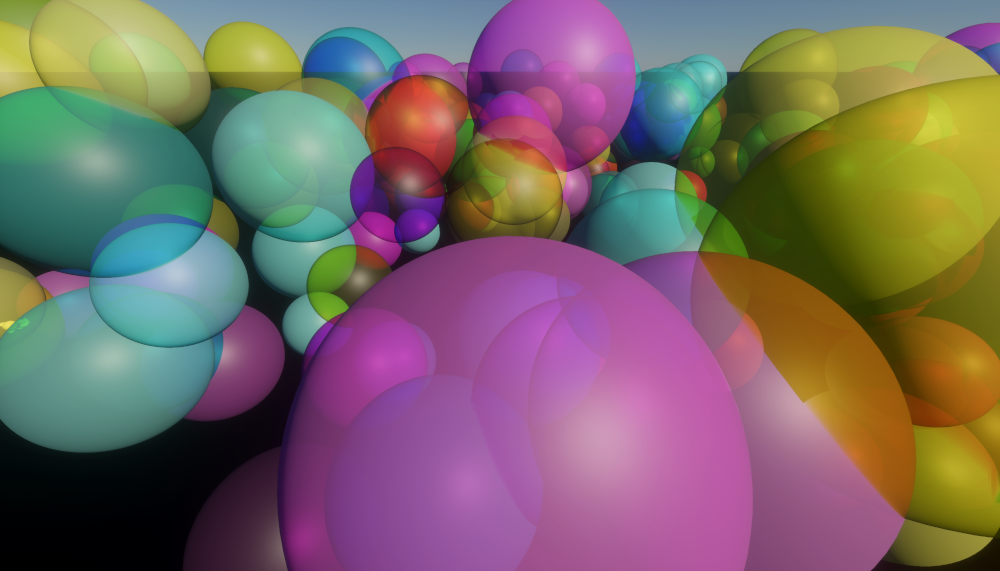
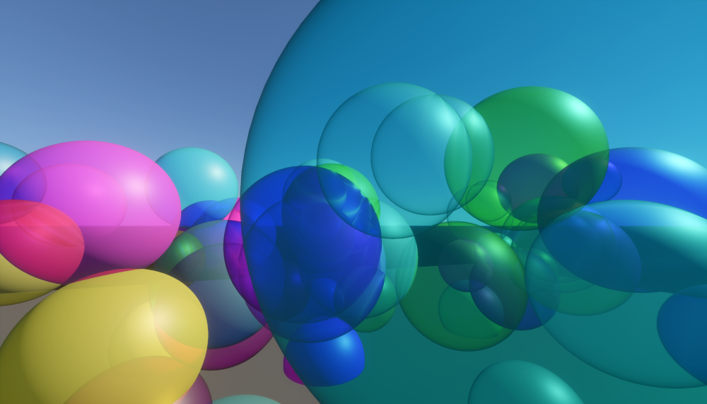
A neat trick that came from a conversation with @adrien-t (thanks! 😊) is to remove the contribution of the surface that’s sampling the transmittance in front of itself, but that also has contributed to transmittance in a previous pass. In this case, there could be some self-occlusion issues because of how the limited number of coefficients represent the function over depth.
The realization here is that, in the shading pass, we can take the generated coefficients and modify them to effectively create a local transmittance-over-depth function that doesn’t include the event that’s currently doing the sampling. Since the coefficients are additive, we can just repeat the logic as if we were to add the coefficients, but subtracting instead.
Here are some screenshots comparing the results when removing the contribution of the surface that’s sampling transmittance or not. These are with any injected noise and denoiser removed, with rank 2, and with a few extra spheres forced to overlap.
| Avoiding Self-Occlusion Off | Avoiding Self-Occlusion On |
 |
 |
 |
 |
 |
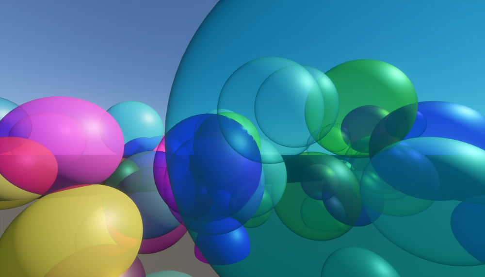 |
Spent a good while trying to find the worst cases of self-occlusion and making a scene that would make them most noticeable. In most cases you aren’t likely to see them as obvious as here, but it’s still a great trick to have in mind and it noticeably improves the quality overall.
Implementing this is slightly simpler once you have merged the two calls to evaluate_wavelet_index into the same loop, so if you have to subtract the contribution of the sampled surface, you only have to do it once per coefficient. Here’s a snippet of how evaluate_wavelets might look like afterwards, note that evaluate_wavelet_index is not necessary now:
template<typename floatN, typename Coefficients_Type, bool REMOVE_SIGNAL = true>
floatN evaluate_wavelets(in Coefficients_Type coefficients, float depth, floatN signal = 0)
{
    floatN scale_coefficient = coefficients.sample(TRANSPARENCY_WAVELET_COEFFICIENT_COUNT - 1);
    if (all(scale_coefficient == 0))
    {
        return 0;
    }
    if (REMOVE_SIGNAL)
    {
        floatN scale_coefficient_addend = mad(signal, -depth, signal);
        scale_coefficient -= scale_coefficient_addend;
    }

    depth *= float(TRANSPARENCY_WAVELET_COEFFICIENT_COUNT-1) / TRANSPARENCY_WAVELET_COEFFICIENT_COUNT;

    float coefficient_depth = depth * TRANSPARENCY_WAVELET_COEFFICIENT_COUNT;
    int index_b = clamp(int(floor(coefficient_depth)), 0, TRANSPARENCY_WAVELET_COEFFICIENT_COUNT - 1);
    bool sample_a = index_b >= 1;
    int index_a = sample_a ? (index_b - 1) : index_b;

    index_b += TRANSPARENCY_WAVELET_COEFFICIENT_COUNT - 1;
    index_a += TRANSPARENCY_WAVELET_COEFFICIENT_COUNT - 1;

    floatN b = scale_coefficient;
    floatN a = sample_a ? scale_coefficient : 0;

    [unroll]
    for (int i = 0; i < (TRANSPARENCY_WAVELET_RANK+1); ++i)
    {
        int power = TRANSPARENCY_WAVELET_RANK - i;

        int new_index_b = (index_b - 1) >> 1;
        int wavelet_sign_b = ((index_b & 1) << 1) - 1;
        floatN coeff_b = coefficients.sample(new_index_b);
        if (REMOVE_SIGNAL)
        {
            float wavelet_phase_b = ((index_b + 1) & 1) * exp2(-power);
            float k = float((new_index_b + 1) & ((1u << power) - 1));
            floatN addend = mad(mad(-exp2(-power), k, depth), wavelet_sign_b, wavelet_phase_b) * exp2(power * 0.5) * signal;
            coeff_b -= addend;
        }
        b -= exp2(float(power) * 0.5) * coeff_b * wavelet_sign_b;
        index_b = new_index_b;

        if (sample_a)
        {
            int new_index_a = (index_a - 1) >> 1;
            int wavelet_sign_a = ((index_a & 1) << 1) - 1;
            floatN coeff_a = (new_index_a == new_index_b) ? coeff_b : coefficients.sample(new_index_a); // No addend here on purpose, the original signal didn't contribute to this coefficient
            a -= exp2(float(power) * 0.5) * coeff_a * wavelet_sign_a;
            index_a = new_index_a;
        }
    }

    float t = coefficient_depth >= TRANSPARENCY_WAVELET_COEFFICIENT_COUNT ? 1.0 : frac(coefficient_depth);

    return lerp(a, b, t);
}
I’ve put all of the code related to removing the contribution of the provided signal under REMOVE_SIGNAL, so it’s both easy to find and potentially to remove if you want just the merged loop code.
Dynamic Rank Selection
Not all scenes have the same transparency complexity and so they could get away with using lower ranks (meaning lower coefficient counts, memory and bandwidth usage) for a similar or even exact result.
We can use the initial depth pass to get an idea of the complexity of the transmittance function for a given pixel or tile of pixels. Then dynamically select a desired rank for that section and allocate that from a shared coefficient pool. If memory and bandwidth is a concern, especially at higher resolutions, this could help with alleviate that issue.
You could even allocate a smaller pool than necessary for the whole screen to be at the max allowed rank. In that case, the rank allocation pass would need to be able to detect overflow and fall back to a lower maximum rank.
Here you can see how in the example scene, the majority of output pixels have either no transparency at all or just one event (green). Only a few areas have two (yellow) or more (red) overlapping surfaces, and these would be the ones that would make use of the higher coefficient counts.
![]()
Overview of the Final Algorithm
Here is the outline of the current algorithm I’m running at the time of writing. It puts together the base idea of generating transmittance and shade later with some of the improvements mentioned above.
The resources that are explicit to this algorithm are the following. Currently all run at native render resolution, that is, the same resolution as the opaque pass:
- Transparency depth buffer: Single
D32_FLOATtexture. - Transparency depth bounds: Single
R16G16_FLOATtexture. - Transparency coefficients array:
R9G9B9E5_SHAREDEXPtexture array of length 8 for rank 2, or length 16 for rank 3. - Transparency lighting buffer: Single
R16G16B16A16_FLOATtexture;
And this is a high level view of what a single frame does to handle transparency:
- Generate depth for the opaque layer (not covered here): In my case this comes from my visibility buffer pass.
- Initialize the transparency buffers:
- The transparency depth buffer is initialized to be a copy of opaque depth.
- The transparency depth bounds min/max are set to $(-\infty, 0)$ (minus infinite because min is inverted so we can max-blend into it).
- The coefficients texture array all gets cleared to zeroes.
- Render transparency depth: Go through all the transparency draws to generate only depth, writing min/max depth to the bounds.
- Render transmittance: Going through all the transparency draws again but generating transmittance, this time generating the coefficients that get added to the coefficient texture array.
- Writing depth at zero transmittance: Look for pixels where transmittance reaches zero and write depth to the transparency depth buffer at that point.
- Shade transparency: Final draw for all transparent surfaces with full shading. This samples the transmittance previously generated and also depth tests against the transparency depth buffer, preventing us from shading surfaces that would have contributed zero to the final result. This renders into the transparency-only lighting buffer.
- Shade the opaque layer (not covered here): Resolving the visibility buffer to have a final opaque layer lighting result. This uses the transparency depth buffer to avoid shading pixels that will be fully covered later.
- Composite the transparency lighting buffer on top of the opaque layer, occluding the opaque layer first via the transmittance at maximum depth.
Note that all three of the rendering passes depth test against the transparency depth buffer. The first two could use the opaque depth, since at that point they are a copy of each other.
I’m also not currently running the denoising pass explicitly on the transparency results before compositing since my current temporal anti-aliasing solution already helps significantly. That said, as I add more complex draws with more overlapping surfaces (such as with particles) I anticipate it being a better idea to enable transparency denoising.
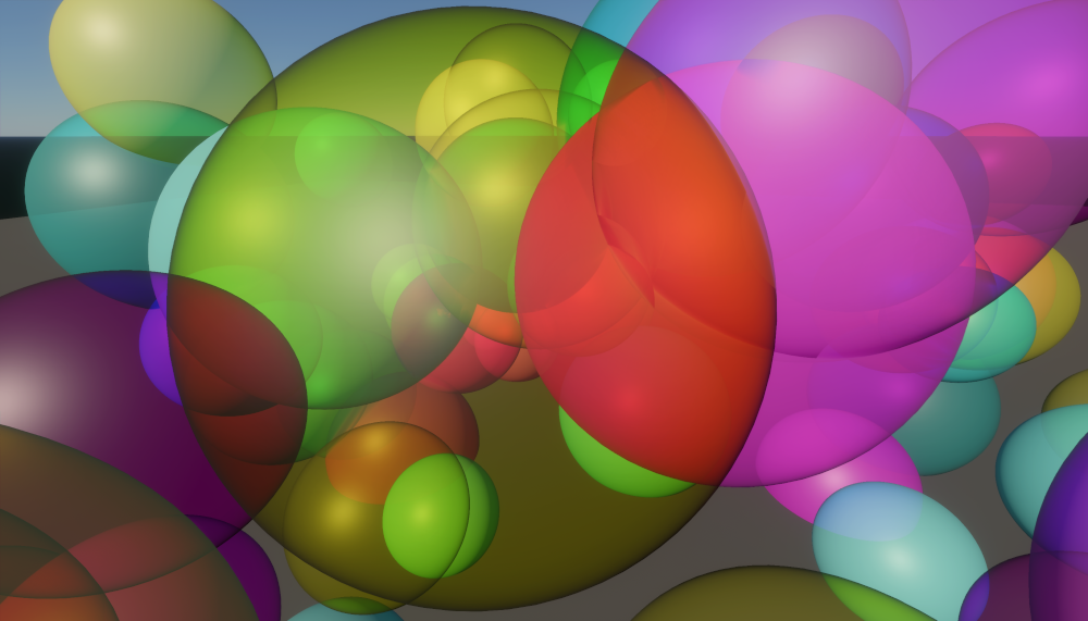
A test that proved useful when implementing this was to force opaque draws to go through this algorithm to verify that both ordering looks correct and there’s no light leaking through that should have been fully occluded. Here’s the example scene with all the balls having $(0,0,0)$ transmittance. You can see how it looks pretty much like opaque rendering would, which is the desired result.
Performance
In the table in this section you can see the performance characteristics of the simple implementation I’m running at the time of writing for the example scene at the beginning of this post. This is running at $2560\times1440$ in a 3080 slightly under-clocked and rendering 200 transparent spheres.
The example scene just has a single directional light which makes the shading pass take a similar amount to transmittance generation, if we add 100 point lights scattered around the spheres we can see how only the shading pass becomes more expensive.
| Rank | Extra Lights | Depth Bounds | Clearing Coefficients | Generating Transmittance | Writing Overdraw Depth | Shading Transparency | Composite Transparency |
|---|---|---|---|---|---|---|---|
| 3 | 0 | 0.13ms | 0.17ms | 0.35ms | 0.06ms | 0.27ms | 0.04ms |
| 3 | 100 | 0.13ms | 0.17ms | 0.35ms | 0.06ms | 0.90ms | 0.04ms |
| 2 | 100 | 0.13ms | 0.09ms | 0.30ms | 0.06ms | 0.87ms | 0.04ms |
| 1 | 100 | 0.13ms | 0.05ms | 0.26ms | 0.05ms | 0.83ms | 0.04ms |
The numbers here aren’t terribly useful, since it heavily depends on how much work you would need to do in the different passes. For example, depending on the amount of vertex work you need to do in each draw, having to do multiple passes might affect your use case differently. Similarly, other types of draws like particles might behave way different.
In this implementation I’m also using the normal and view direction to vary the transmittance of the surface, this makes that pass need to do a significant amount of work more compared to just sampling transmittance and outputting it. If I remove using the normal for the transmittance the pass goes from 0.35ms to 0.17ms. This is a good example of the variability in cost depending on how much work each of the steps requires for a given use case.
As mentioned above, you could even do transparency at a lower resolution and upscale when compositing, or even do dynamic resolution on transparency.
Changing rank to 2 is also a very solid option and in this scene is essentially imperceptible, although the more surfaces contribute to a single pixel the more you would be able to see the difference. However, by adding noise and possibly a denoiser pass before compositing, the results might be indistinguishable in the majority of scenes.
I also haven’t made any real attempts at heavily optimizing this implementation. I might end up doing a deep dive into it with Nsight or Radeon GPU Profiler, which could be a good candidate to add in a further post about this technique!
And just because I find it satisfying to look at, here is the scene with the 100 lights:
Conclusion & Final Comments
I hope this motivates some people to go and implement some form of OIT and further develop these or new techniques! On my side I look forward to do further blog posts expanding on the ideas presented here or investigating new ones.
I think it would be really interesting to do a continuation of this post with more complex scenes, including elements like particles or volumetrics. It took me a while to write this post and it’s gotten longer than expected, so even now there’s interesting parts I would like to add about good ways of implementing volumetrics into this, marrying transparency with (separate? 🙃) temporal filters, etc. That said, I should eventually stop writing this at some point, and now feels like the right time.
Let me know if any of this is helpful, if there’s any questions, etc. It’s the first post on this site so there may or may not be a comments section. But regardless you can find me in most places as some variation of “osor_io” or “osor-io” and there should be links at the bottom of the page as well.
Cheers! 🍻